Every Single Component You Need to Know About
Read this story for free: link
It is one thing to train a machine learning model, maybe achieve state-of-the-art accuracy on a benchmark dataset. But deploying that model, making it serve millions of users, process terabytes of data, and operate reliably 24/7 is a very different challenge.
From the start, every part of training and deploying a machine learning model, each stage requires careful planning and the right tools.
Building and running an AI system from early development to full deployment is where …
Strong software development skills become important, a gap where many AI engineers fall short
In this blog, we will explore each development stage required to build a large-scale AI system capable of creating LLMs, multimodal models, and various other AI products. How each development stage relate to one another, and their individual responsibilities.
Special thanks to
from Meta for the guidance provided in his GitHub repo.
Our table of contents is organized by phases. Feel free to explore each phase as you go.
Phase I: Systems and Hardware for AI
Phase II: Advanced Model Training Techniques
- Strategies for Optimizing Neural Network Training
- Frameworks and Tools for Large-Scale Training
- Scaling Up with TensorFlow and PyTorch
- Model Scaling and Efficient Processing
Phase III: Advanced Model Inference Techniques
- Efficient Inference at Scale
- Efficient Inference at Scale
- Managing Latency and Throughput for Real-Time Applications
- Edge AI and Mobile Deployment
Phase IV: Performance Analysis and Optimization
- Diagnosing System Bottlenecks
- Operationalizing AI Model
- Debugging AI Systems: Tools and Methodologies
- CI/CD Pipelines for Machine Learning
- Conclusion
Phase I: Systems and Hardware for AI
The very first step in building a large-scale AI system is choosing the right hardware. It affects how fast your models run, how much money you spend, and how much energy everything uses.
In this section, we will discuss the different hardware systems available, along with how to make them cost and energy-efficient.
Compute Hardware for AI
The three most common types of hardware widely used for training or other AI tasks are:
Zoom image will be displayed
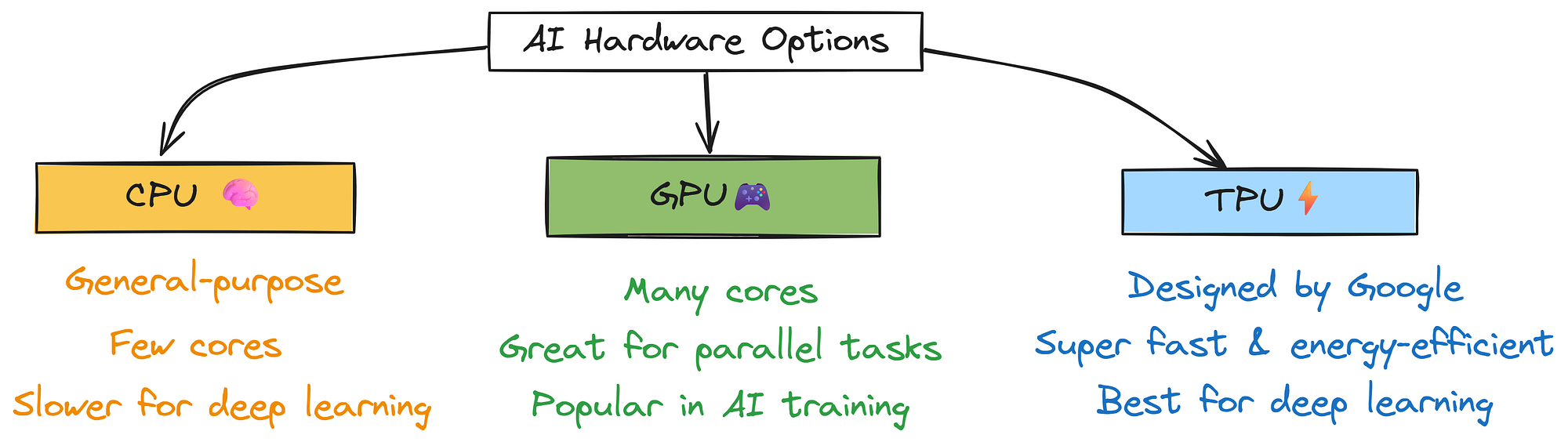
AI Hardware Availability (Created by )
- CPUs (Central Processing Units) They are good at doing lots of different tasks, but they don’t have many cores, so they can be slower for deep learning or large AI jobs that need lots of parallel processing.
- GPUs (Graphics Processing Units) were originally built to handle video and graphics, but now they are a favorite for AI. Because they have many more cores than CPUs, which means they can process a lot of things at the same time, perfect for training and running AI models.
- TPUs (Tensor Processing Units) are special chips made by Google just for deep learning. They are really fast, super efficient, and use less energy. That makes them great for big, complex AI tasks.
You can learn more here: https://cloud.google.com/tpu
But recently, due to the growing demand for AI, some new types of hardware have also been introduced.
Zoom image will be displayed
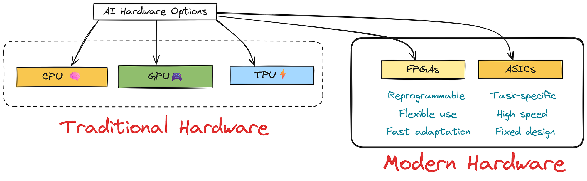
Modern Hardware (Created by )
- One great example is FPGAs (Field-Programmable Gate Arrays). These chips are special because they can be reprogrammed to fit different AI tasks. They give you the flexibility to fine-tune performance based on what your model needs, which can be super useful in fast-changing AI projects.
- Then there are ASICs (Application-Specific Integrated Circuits). These aren’t general-purpose like CPUs or even FPGAs. Instead, they are designed for one thing: running AI models as fast and efficiently as possible. Because they’re built with a specific job in mind like powering neural networks, they save energy and run really fast.
You can read this story for more detail:
When it comes to choosing hardware, directly jumping to GPUs is not always the correct approach, as we often assume they automatically improve performance whether for data preprocessing, fine tuning, or LLM inference.
However, performance strongly depends on …
Model architecture + infrastructure choice
- For the AI architecture side, one helpful technique is model quantization, which many modern open source model API providers such as Together AI or Nebius AI are already using. This means reducing how much detail your AI model uses when doing calculations like using smaller numbers (e.g., 8-bit instead of 32-bit).
- On the infrastructure side, cloud services and virtualization are often the best solutions. Instead of purchasing expensive hardware, you can rent powerful machines from providers like AWS, Google Cloud, or Azure. This gives you the flexibility to scale up or down depending on your project, which saves money and avoids waste.
Take a look at the comparison graph from Google that shows different model architectures perform across various GPUs.
Zoom image will be displayed
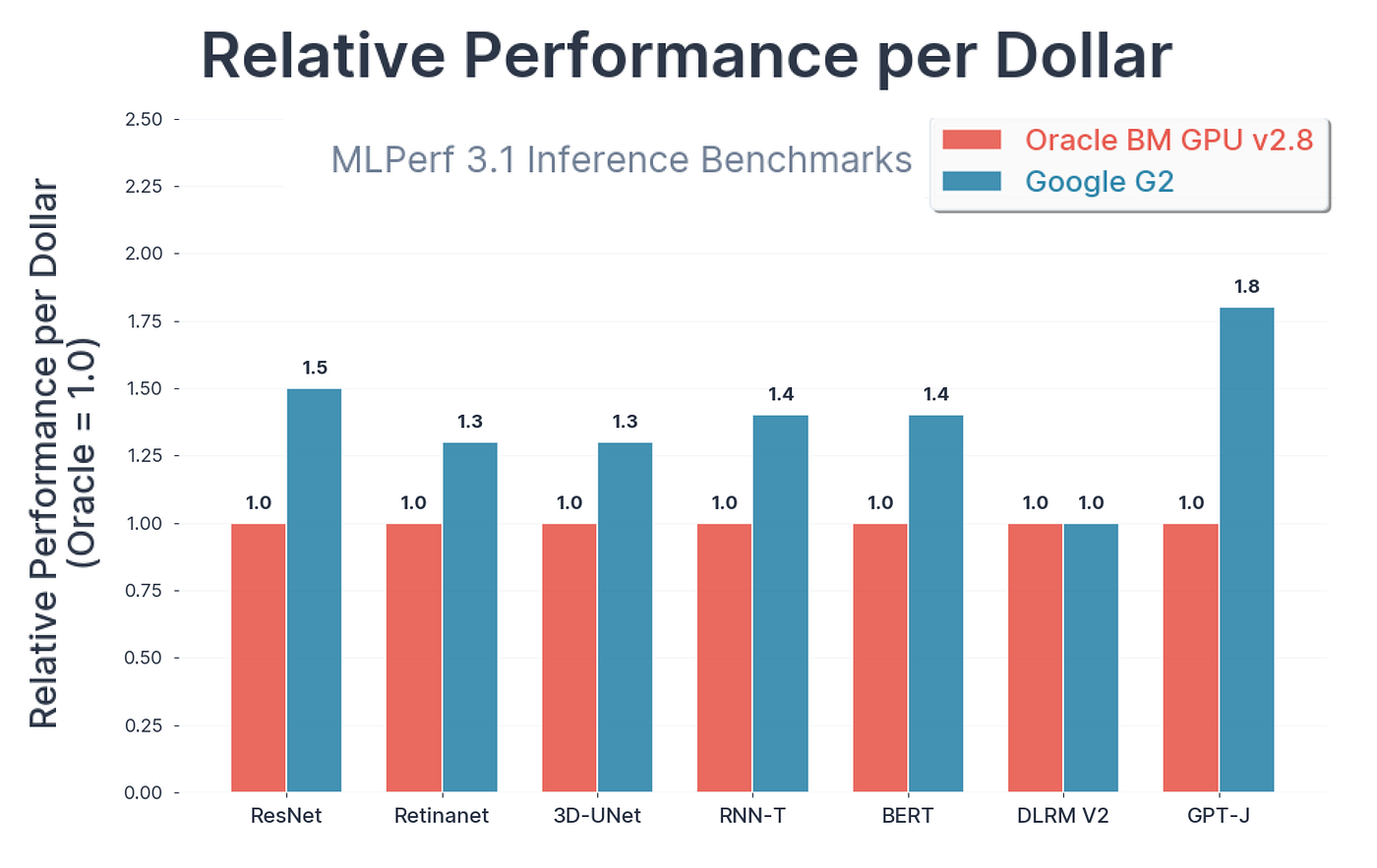
Performance Comparison (Created by — Google Comparison Article)
Google tested this on MLPerf 3.1 benchmark (Mostly used for how fast systems can process inputs).
- The A3 VM, which uses a powerful H100 GPU, is much faster than the older A2 VM between 1.7 to 3.9 times faster for tough AI jobs.
- The G2 VM, which uses the L4 GPU, is a good option if you’re looking to save money while still getting solid AI performance.
- Tests show that the L4 GPU can deliver up to 1.8 times better performance for every dollar spent compared to similar cloud services.
Companies like Bending Spoons are already using G2 VMs to bring new AI features to their users efficiently.
Distributed Systems for AI
Once you choses the optimized hardware and your model architecture based on your requirements, we move onto next stage, which involves how you plan for distributional system for AI.
The main principle of a distributed system is …
Splitting a large task into smaller parts and having multiple computers work on them simultaneously.
In AI, this speeds up data processing and model training by sharing the workload.
So, to create a distributed system, we need to keep in mind some important factors. Let’s visualize it first and then understand its flow.
Zoom image will be displayed

Distributed AI System (From Sina Torfi — Open Source)
There are various factors we need to keep in mind while applying the distribution logic into our AI system. Let’s see how the flow goes:
- First, we need to understand the scale. Are we dealing with hundreds, thousands, or millions of data points? Knowing this early helps us plan the system to grow smoothly.
- Next, we choose the right tools. Depending on the size and type of the project, we need the right mix of processing power, memory, and communication methods. Cloud platforms make this much easier to manage.
- Then, we make sure everything works together. Different parts of the system might need to run in parallel or on separate machines. Our goal is to avoid slowdowns and keep things running smoothly.
- After that, we keep things flexible. Instead of manually adjusting resources, we automate it. Tools like Kubernetes help the system adjust automatically as the load changes.
- We also need to monitor performance. Keeping an eye on the system helps us spot issues early, whether it’s uneven data distribution or a network bottleneck.
- Finally, we make sure everything stays in sync. As the system scales, it is critical that data and models stay consistent across all parts.
Optimizing Networking
Once you decide on the distribution part of your AI system, you need to ensure that all components are properly connected.
They must be able to communicate with each other smoothly and without any hiccups
If the distributed components fail to communicate effectively, it can break your training or production code.
Let’s see how to make the conversation flow without breaking it:
Zoom image will be displayed
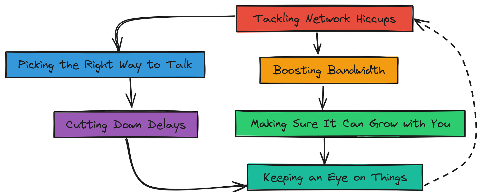
Network Optimization for Distributed System (Created by )
Let’s break it down:
- First, we look for potential slowdowns. Delays, limited capacity, or lost data can seriously impact performance, so it’s important to identify these risks early.
- Then, we reduce the delay. To speed things up, we use faster connections, place machines close together, or even shift some processing to the edge.
- Next, we increase the bandwidth. A narrow network path causes traffic jams. We solve this by compressing data, prioritizing important info, or upgrading the network.
- After that, we choose the right communication methods. Some protocols handle large loads better than others. Picking the right one ensures your system runs fast and efficiently.
- We also plan for future growth. As the system scales, the network must keep up. Using flexible setups that can grow as needed is key.
- Finally, we monitor the network. Regular checks help us spot problems early. Monitoring tools can alert us to issues before they slow things down.
Storage Solutions for AI
So, after you have decided on the hardware for training or inferencing and the distribution logic behind it, the next thing you need is storage to save your trained model as well as the data from user conversations with your AI model.
The way we store data must be smart for today and ready for more data tomorrow
Zoom image will be displayed

Growing Demand of AI Storage (From Market US)
We have three types of data storage system:
Zoom image will be displayed
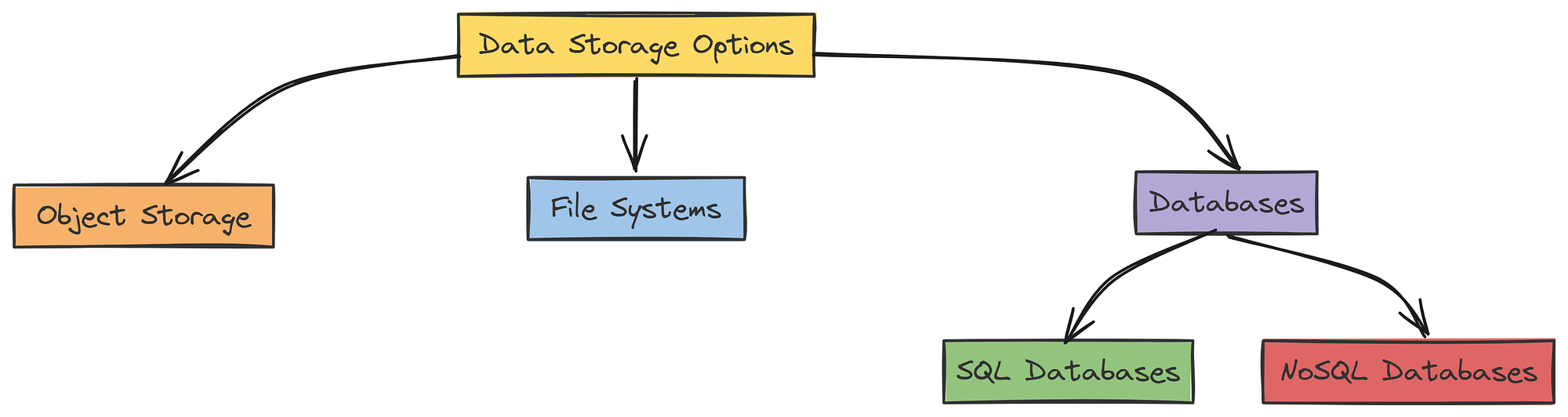
Data Storage Options (Created by )
- Object storage works best for big data. It’s where you can keep adding files without stressing over structure. It’s perfect when your data comes from many sources and needs to be pulled together later.
- File systems are better for smaller, organized setups. They are kind of a folders on your computer. They help keep things neat and are ideal when your data is limited and well-structured.
While the third type that is Databases, are useful when your data has structure. Here’s how to choose the right type:
- SQL databases are great for organized, connected data. Use them when your data has clear relationships like users, orders, and products. They’re perfect for complex tasks where accuracy and consistency matter.
- NoSQL databases work well with flexible or changing data. If your data doesn’t fit neatly into tables or grows quickly, NoSQL options like MongoDB or Cassandra offer the freedom and scale you need.
Though the tools are not the only thing that matters but it’s also important how you use them:
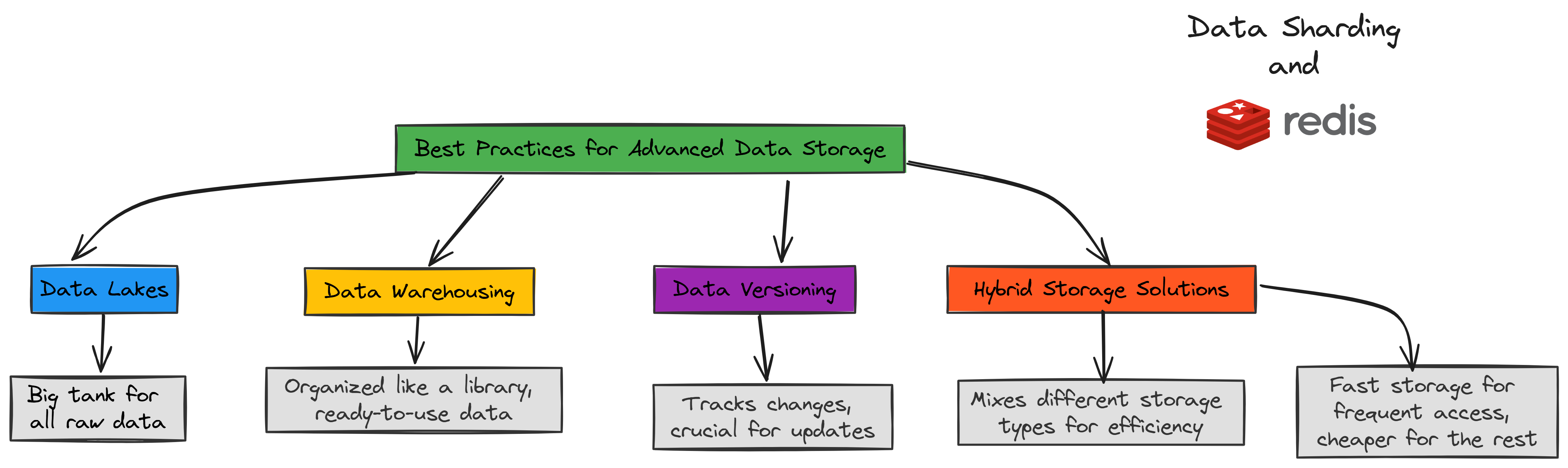
Best Practices for Data Storage (Created by )
- Data lakes hold everything in raw form. It is a giant container for all kinds of data that you can sort and process later.
- Data warehouses store clean, ready-to-use data. This is like a well-organized library where you can quickly find exactly what you need.
- Data versioning keeps track of changes. This is important when updating models or working with data that changes over time. It helps keep things organized and prevents mistakes.
- Hybrid storage combines speed and savings. You use fast storage for data you need often and cheaper storage for the rest. This way you save money while still getting quick access when necessary.
Fast data access is key for AI performance.
Use in-memory stores like Redis for quick retrieval, and apply data sharding to distribute load and prevent slowdowns.
At some point, you need to decide what storage setup works best: cloud, on-premises, or a mix of both.
Zoom image will be displayed
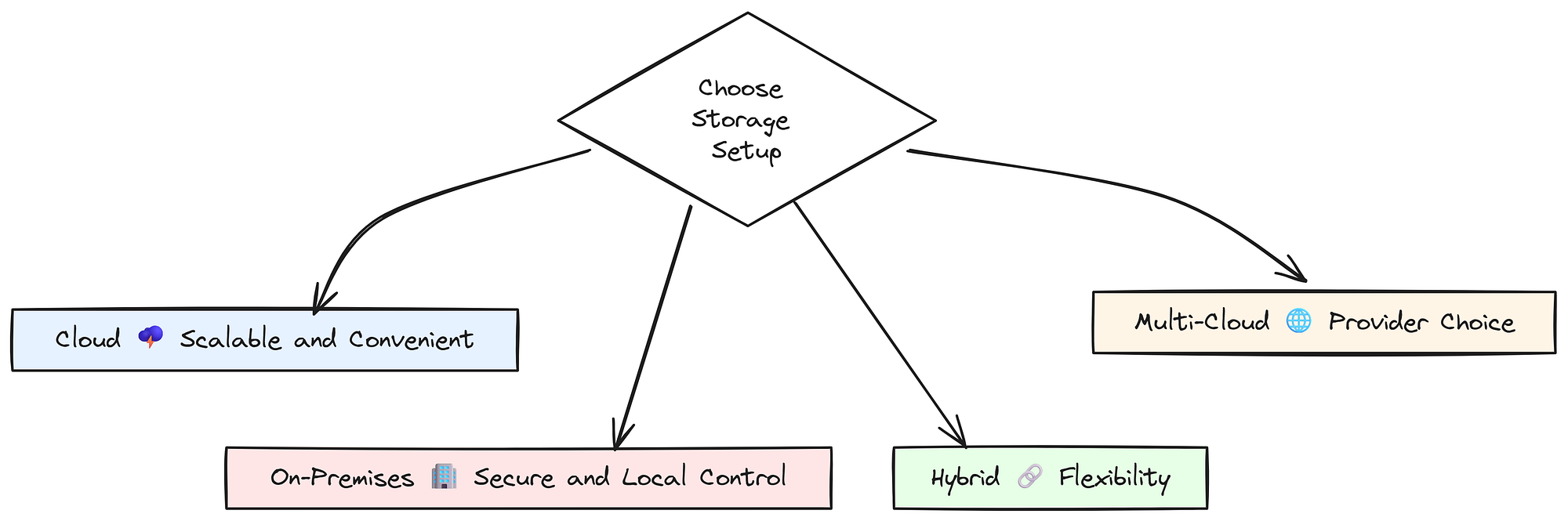
Cloud vs on-premises (Created by )
- Hybrid storage gives you flexibility. You can keep sensitive data on your own servers while using the cloud for everything else. This helps balance security and scalability.
- Multi-cloud strategies offer more choice. By using multiple cloud providers, you avoid being locked into one. It’s like having different menus to pick from, depending on what you need.
Phase II: Advanced Model Training Techniques
So far, we have covered hardware, storage, and how to make the most of them. Now it’s time to look at how training techniques work and how we can optimize them too.
Strategies for Optimizing Neural Network Training
AI models are often built on neural networks, and while many start with basic gradient descent, there are more advanced options that perform better in real-world scenarios.
Zoom image will be displayed
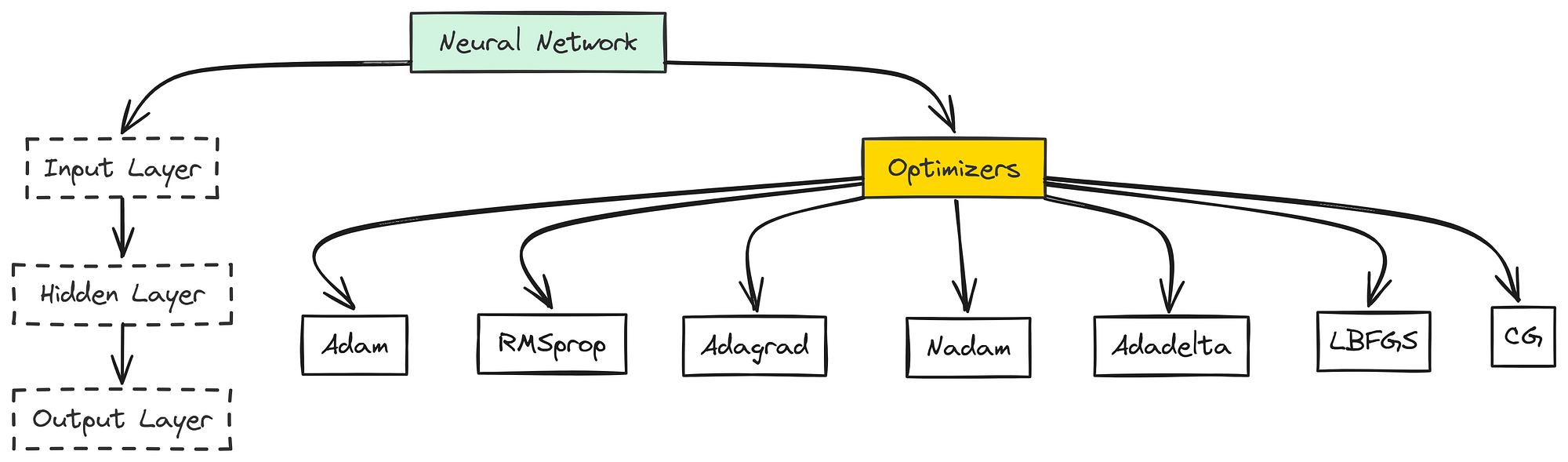
Optimizing Neural Networks (Created by )
Adam optimization is a smart choice. It combines the strengths of AdaGrad and RMSprop. It handles noisy data and sparse gradients well, making it a popular default choice.
<span id="5d20" data-selectable-paragraph="">optimizer = optim.Adam(model.parameters(), lr=<span>0.001</span>)</span>
RMSprop helps with learning stability. It adjusts the learning rate based on recent gradient behavior and works well for non-stationary problems.
<span id="614e" data-selectable-paragraph="">optimizer = optim.RMSprop(model.parameters(), lr=<span>0.001</span>, alpha=<span>0.99</span>)</span>
Adagrad adapts to your data. It changes the learning rate for each parameter, which is great for sparse data but can cause the learning rate to shrink too much over time.
<span id="5d9c" data-selectable-paragraph="">optimizer = optim.Adagrad(model.parameters(), lr=<span>0.01</span>)</span>
Let’s have a simple table that will give us a high level overview of what optimizer we have and where they fit together.
So, this comparison can help machine learning engineers decide which optimizer to choose.
We can safely start with Adam. Although there are differences among optimizers, it’s important to begin with something practical and gain some initial insights.
Frameworks and Tools for Large-Scale Training
Next come the regularization techniques, which are critical for preventing overfitting and ensuring that models generalize well to new data. Here are some common ways to help your model generalize well to new data.
Regularization techniques (Created by )
L2 regularization with weight decay helps by discouraging large weights, keeping the model simpler.
<span id="9b87" data-selectable-paragraph="">optimizer = optim.Adam(model.parameters(), lr=<span>0.001</span>, weight_decay=<span>1e-5</span>)</span>
Dropout layers in the model randomly dropping neurons during training makes the model less likely to overfit.
<span id="dc0f" data-selectable-paragraph=""><span>class</span> <span>MyModel</span>(nn.Module):<br> <span>def</span> <span>__init__</span>(<span>self</span>):<br> <span>super</span>(MyModel, self).__init__()<br> <br> self.layer1 = nn.Linear(<span>784</span>, <span>256</span>)<br> <br> <br> self.dropout = nn.Dropout(<span>0.5</span>)<br> <br> <br> self.layer2 = nn.Linear(<span>256</span>, <span>10</span>)<br><br> <span>def</span> <span>forward</span>(<span>self, x</span>):<br> <br> x = self.layer1(x)<br> <br> <br> x = self.dropout(x)<br> <br> <br> x = self.layer2(x)<br> <br> <span>return</span> x</span>
Early stopping based on validation loss. If the validation loss stops improving, there’s no point in training further.
<span id="5638" data-selectable-paragraph="">best_loss = <span>float</span>(<span>'inf'</span>) <br>patience = <span>10</span> <br>trigger_times = <span>0</span> <br><br><span>for</span> epoch <span>in</span> <span>range</span>(max_epochs):<br> val_loss = validate(model, val_loader) <br><br> <span>if</span> val_loss < best_loss:<br> best_loss = val_loss <br> trigger_times = <span>0</span> <br> <span>else</span>:<br> trigger_times += <span>1</span> <br><br> <span>if</span> trigger_times >= patience:<br> <span>print</span>(<span>'Early stopping'</span>) <br> <span>break</span></span>
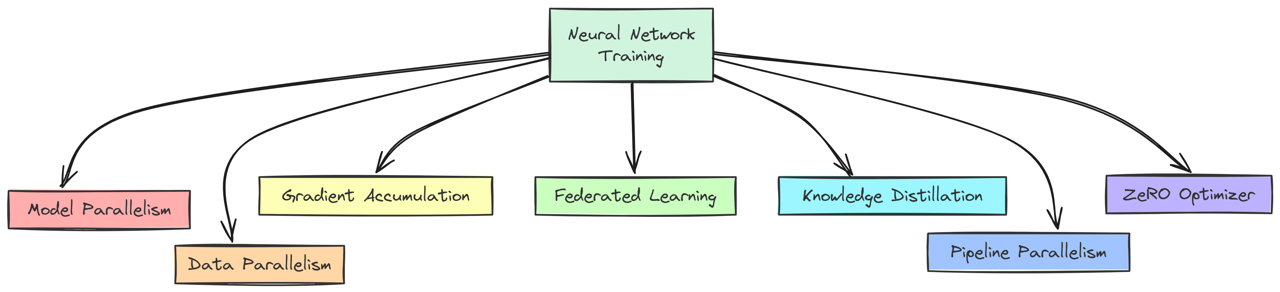
Handling very large models introduces new challenges. Here are some ways to make it manageable.
Model parallelism splits the model across GPUs. Different parts of the model are processed on different devices.
<span id="4239" data-selectable-paragraph=""><br>self.seq1 = nn.Sequential(<br> <br>).to(<span>'cuda:0'</span>)<br><br><br>self.seq2 = nn.Sequential(<br> <br>).to(<span>'cuda:1'</span>)<br><br><br>self.fc = nn.Linear(...).to(<span>'cuda:1'</span>)</span>
Data parallelism spreads the data across GPUs. PyTorch DataParallel automatically manages this process.
<span id="4694" data-selectable-paragraph="">model = DataParallel(MyModel())<br>model.to(<span>'cuda'</span>)</span>
Gradient accumulation allows for bigger batches. It helps when memory is limited by accumulating gradients before updating.
<span id="38c7" data-selectable-paragraph=""><br>optimizer.zero_grad()<br><br><span>for</span> i, (inputs, labels) <span>in</span> <span>enumerate</span>(training_set):<br> <br> outputs = model(inputs)<br><br> <br> loss = loss_function(outputs, labels)<br><br> <br> loss.backward()<br><br> <br> <span>if</span> (i + <span>1</span>) % accumulation_steps == <span>0</span>:<br> optimizer.step() <br> optimizer.zero_grad() </span>
Federated learning keeps data on local devices. Models are trained on devices separately, and only the updates are shared.
<span id="bb01" data-selectable-paragraph=""><span>for</span> <span>round</span> <span>in</span> <span>range</span>(num_rounds):<br> model_updates = [] <br><br> <br> <span>for</span> device <span>in</span> devices:<br> updated_model = train_on_device(model, device.data) <br> model_updates.append(updated_model.get_weights()) <br><br> <br> model.set_weights(aggregate(model_updates))</span>
To make large models more efficient without losing too much performance, knowledge distillation is a great approach.
Train a small student model using a large teacher model. This helps reduce size while keeping good accuracy.
<span id="19ce" data-selectable-paragraph=""><span>def</span> <span>knowledge_distillation_loss</span>(<span>outputs, labels, teacher_outputs, temp=<span>2.0</span>, alpha=<span>0.5</span></span>):<br> <br> hard_loss = F.cross_entropy(outputs, labels)<br><br> <br> <br> soft_loss = F.kl_div(<br> F.log_softmax(outputs / temp, dim=<span>1</span>), <br> F.softmax(teacher_outputs / temp, dim=<span>1</span>), <br> reduction=<span>'batchmean'</span> <br> )<br><br> <br> <br> <span>return</span> alpha * hard_loss + (<span>1</span> - alpha) * soft_loss * (temp ** <span>2</span>)</span>
By combining the right optimizers, regularization methods, and training strategies, we can build models that are both powerful and efficient, even at scale.
Let’s have a comparison table for this to gain a much clearer understanding.
Scaling Up with TensorFlow and PyTorch
Frameworks also play a big role when working with AI at scale. Here are some popular options:
Zoom image will be displayed
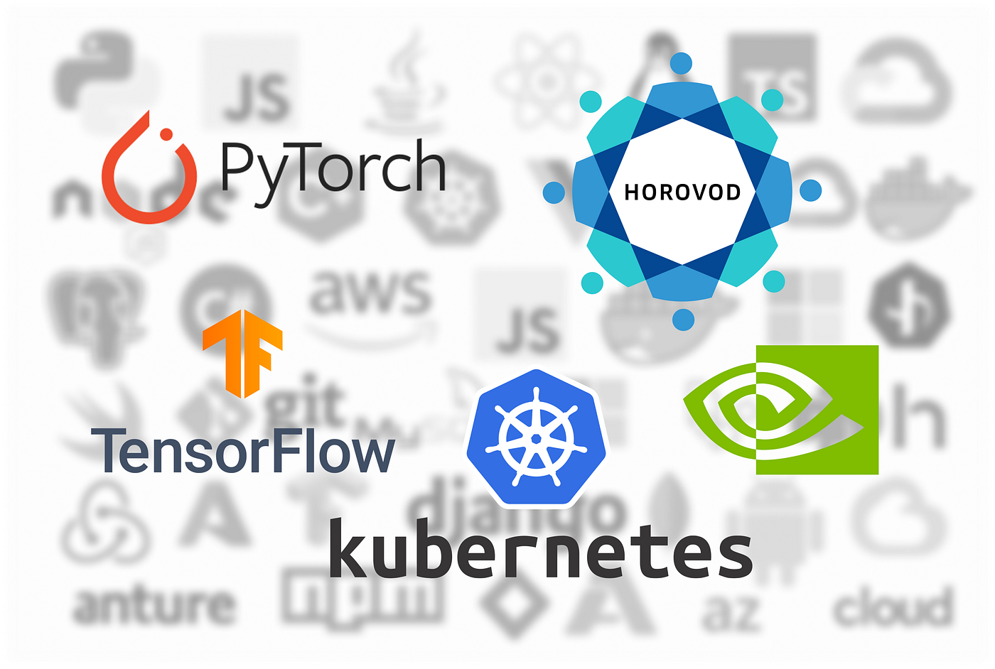
Most Important Frameworks (Created by )
- TensorFlow offers TensorFlow Distributed Strategies to help scale training efficiently across GPUs and TPUs.
- PyTorch is known for PyTorch Distributed, supporting scaling across multiple GPUs and multiple machines.
- Horovod works with TensorFlow, PyTorch, and Keras to improve scalability on GPUs and CPUs.
- Kubernetes helps deploy and manage AI workloads smoothly when running at scale.
- CUDA and cuDNN accelerate GPU computing and deep learning performance.
- NeMo focuses on building speech and natural language processing models.
Model Scaling and Efficient Processing
Scaling models is key to handling big datasets and complex tasks. Let’s explore simple ways to parallelize models and data, process batches smartly, and handle training challenges.
Model Parallelism, We can split our model across devices when it’s too big for one GPU. You can divide by layers (vertical) or parts of layers (horizontal). The goal is to reduce data moving between devices.
<span id="cb4c" data-selectable-paragraph=""><span>import</span> torch<br><span>import</span> torch.nn <span>as</span> nn<br><br><br><span>class</span> <span>SimpleModel</span>(nn.Module):<br> <span>def</span> <span>__init__</span>(<span>self</span>):<br> <span>super</span>(SimpleModel, self).__init__()<br> self.layer1 = nn.Linear(<span>10</span>, <span>20</span>)<br> self.relu = nn.ReLU()<br> self.layer2 = nn.Linear(<span>20</span>, <span>10</span>)<br> self.layer3 = nn.Linear(<span>10</span>, <span>5</span>)<br><br> <span>def</span> <span>forward</span>(<span>self, x</span>):<br> <br> x = self.layer1(x)<br> x = self.relu(x)<br><br> <br> x = x.to(device2)<br> <br> x = self.layer2(x)<br> x = self.relu(x)<br> x = self.layer3(x)<br> <span>return</span> x<br><br><br>model = SimpleModel()<br><br><br>device1 = torch.device(<span>'cuda:0'</span>)<br>device2 = torch.device(<span>'cuda:1'</span>)<br><br><br>model.layer1.to(device1)<br>model.relu.to(device1) <br>model.layer2.to(device2)<br>model.layer3.to(device2)<br><br><br>x = torch.randn(<span>1</span>, <span>10</span>).to(device1)<br><br><br>output = model(x)<br><br></span>
We can use fast communication libraries like NCCL to reduce delays when moving data and torch.cuda.synchronize() to make sure devices finish tasks in order.
<span id="4374" data-selectable-paragraph=""><span>import</span> torch<br><span>import</span> torch.distributed <span>as</span> dist<br><br><br><span>def</span> <span>init_process</span>(<span>rank, size, backend=<span>'nccl'</span></span>):<br> dist.init_process_group(backend, rank=rank, world_size=size)<br><br>world_size = <span>4</span><br><span>for</span> i <span>in</span> <span>range</span>(world_size):<br> init_process(rank=i, size=world_size, backend=<span>'nccl'</span>)<br><br><br><br><br><span>def</span> <span>synchronize_devices</span>(<span>devices</span>):<br> <span>for</span> device <span>in</span> devices:<br> <span>if</span> <span>'cuda'</span> <span>in</span> <span>str</span>(device):<br> torch.cuda.synchronize(device)<br><br>device1 = torch.device(<span>'cuda:0'</span>)<br>device2 = torch.device(<span>'cuda:2'</span>)<br>synchronize_devices([device1, device2])</span>
Data Parallelism, We can run the same model on different data chunks across multiple devices. This is useful when the model fits on a single GPU, but we want to process more data in parallel.
<span id="b09a" data-selectable-paragraph=""><span>import</span> torch<br><span>import</span> torch.distributed <span>as</span> dist<br><span>from</span> torch.nn.parallel <span>import</span> DistributedDataParallel <span>as</span> DDP<br><span>from</span> torch.utils.data <span>import</span> DataLoader, Dataset, DistributedSampler<br><br><br><span>class</span> <span>CustomDataset</span>(<span>Dataset</span>):<br> <span>def</span> <span>__init__</span>(<span>self, data</span>):<br> self.data = data<br> <br> <span>def</span> <span>__len__</span>(<span>self</span>):<br> <span>return</span> <span>len</span>(self.data)<br> <br> <span>def</span> <span>__getitem__</span>(<span>self, idx</span>):<br> <span>return</span> self.data[idx]<br><br><br><span>def</span> <span>setup</span>(<span>rank, world_size</span>):<br> dist.init_process_group(backend=<span>'nccl'</span>, rank=rank, world_size=world_size)<br> torch.cuda.set_device(rank)<br><br><br><span>def</span> <span>get_dataloader</span>(<span>dataset, batch_size, rank, world_size</span>):<br> sampler = DistributedSampler(dataset, num_replicas=world_size, rank=rank)<br> <span>return</span> DataLoader(dataset, batch_size=batch_size, sampler=sampler)<br><br><br>rank = <span>0</span><br>world_size = <span>2</span><br>setup(rank, world_size)<br><br>dataset = CustomDataset(torch.arange(<span>1000</span>))<br>dataloader = get_dataloader(dataset, batch_size=<span>32</span>, rank=rank, world_size=world_size)<br><br>model = SimpleModel().to(rank)<br>model = DDP(model, device_ids=[rank])</span>
After the backward pass, DDP syncs gradients across devices so model weights stay the same.
We can also reduce communication load with gradient compression. Here’s a simple version using 8-bit quantization:
<span id="8ccb" data-selectable-paragraph=""><span>def</span> <span>quantize_gradients</span>(<span>model, bits=<span>8</span></span>):<br> q_level = <span>2</span>**bits - <span>1</span> <br><br> <span>for</span> param <span>in</span> model.parameters():<br> <span>if</span> param.grad <span>is</span> <span>not</span> <span>None</span>:<br> grad = param.grad.data <br><br> <br> min_val, max_val = grad.<span>min</span>(), grad.<span>max</span>()<br><br> <br> grad_norm = (grad - min_val) / (max_val - min_val + <span>1e-8</span>) * q_level<br><br> <br> grad_quant = torch.<span>round</span>(grad_norm)<br><br> <br> grad_dequant = grad_quant / q_level * (max_val - min_val) + min_val<br><br> <br> param.grad.data = grad_dequant</span>
Efficient Batch Processing, We can improve speed and memory usage by adjusting how batches are handled.
- Mixed Precision Training uses half-precision (float16) for faster compute:
<span id="3b62" data-selectable-paragraph="">scaler = GradScaler() <br><br><span>for</span> data, target <span>in</span> dataloader:<br> optimizer.zero_grad() <br><br> <span>with</span> autocast(): <br> output = model(data) <br> loss = loss_fn(output, target) <br><br> scaler.scale(loss).backward() <br> scaler.step(optimizer) <br> scaler.update() </span>
- Gradient Accumulation helps if your GPU can’t handle large batches:
<span id="fe7e" data-selectable-paragraph="">optimizer.zero_grad()<br>accum_steps = <span>4</span><br><br><span>for</span> i, (data, target) <span>in</span> <span>enumerate</span>(dataloader):<br> output = model(data)<br> <br> <br> loss = loss_fn(output, target) / accum_steps<br> loss.backward()<br><br> <br> <span>if</span> (i + <span>1</span>) % accum_steps == <span>0</span>:<br> optimizer.step()<br> optimizer.zero_grad()<br><br><br><span>if</span> (i + <span>1</span>) % accum_steps != <span>0</span>:<br> optimizer.step()<br> optimizer.zero_grad()</span>
Let’s understand a basic difference between Synchronous and Asynchronous training difference:
Synchronous Training, All workers wait to exchange gradients before updating weights. Ensures consistent model but slowest worker slows everyone down.
- Gradient averaging
- Adaptive batch sizes
- Predictive wait-time scheduling
Asynchronous Training Workers update weights without waiting. Speeds things up but gradients may be stale.
- Use stale gradient correction
- Dynamically adjust learning rate
- Maintain model versioning to track updates
So, what we have learned so far, let’s summarize it in a table:
Phase III: Advanced Model Inference Techniques
When we deploy ML models and millions of people use them, it definitely requires an efficient inference approach to make it easily accessible to all users.
We often encounter scenarios where resources are not as easily available as we would like. In this section, we will explore various techniques and strategies that can help us make inference more optimized and effective.
Efficient Inference at Scale
Model Quantization helps shrink your model and speed up inference by reducing the precision of its numbers like going from 32-bit floats to 8-bit integers. This means smaller models and faster compute, but watch out for some drop in accuracy.
There are two main types:
Zoom image will be displayed
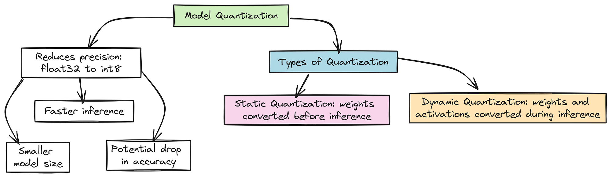
Types of Quantization (Created by )
- Static Quantization: Convert weights to low precision before running the model.
- Dynamic Quantization: Convert weights and activations on the fly during inference, balancing speed and flexibility.
Here’s how to do dynamic quantization with PyTorch on a ResNet18 model:
<span id="75fe" data-selectable-paragraph=""><br><span>import</span> torch<br><span>from</span> torchvision.models <span>import</span> resnet18<br><br><br>model = resnet18(pretrained=<span>True</span>)<br>model.<span>eval</span>() <br><br><br>quantized_model = torch.quantization.quantize_dynamic(<br> model, {torch.nn.Linear, torch.nn.Conv2d}, dtype=torch.qint8<br>)<br><br><br><span>print</span>(quantized_model)</span>
There are two most commonly used training techniques that play an important role in saving disk space, memory, and most importantly, cost.
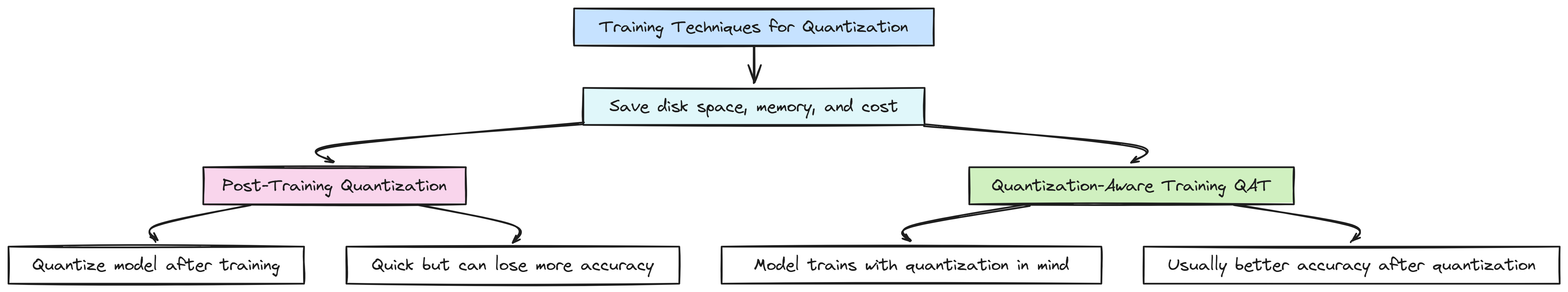
Types of Training Quantization (Created by )
- Post-Training Quantization: You quantize your model after training. It’s quick but can cause more accuracy loss because the model wasn’t trained knowing it would use lower precision.
- Quantization-Aware Training (QAT): The model learns with quantization in mind during training, so it adapts and usually keeps better accuracy after quantization.
Here’s how you do QAT with PyTorch on a ResNet18 model:
<span id="d3ac" data-selectable-paragraph=""><span>import</span> torch<br><span>from</span> torchvision.models <span>import</span> resnet18<br><span>import</span> torch.quantization<br><br>model = resnet18(pretrained=<span>True</span>)<br>model.train()<br><br><br>model = torch.quantization.fuse_modules(model, [[<span>'conv1'</span>, <span>'bn1'</span>, <span>'relu'</span>]])<br><br><br>model.qconfig = torch.quantization.get_default_qat_qconfig(<span>'fbgemm'</span>)<br><br><br>torch.quantization.prepare_qat(model, inplace=<span>True</span>)<br><br><br><br><br>torch.quantization.convert(model, inplace=<span>True</span>)<br><br><span>print</span>(model)</span>
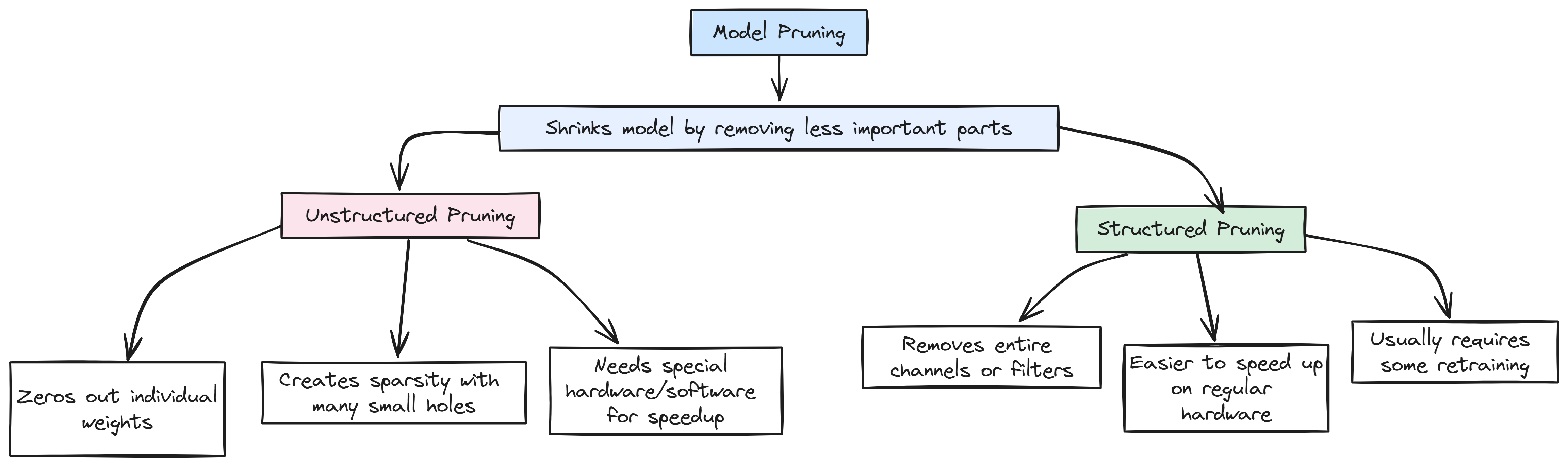
Model Pruning helps shrink models by removing less important parts — either by zeroing out individual weights or cutting out whole neurons or channels.
Model Pruning (Created by )
- Unstructured Pruning: Zeros out individual weights (lots of tiny “holes” in the model). It can make models sparse but often needs special hardware/software to get speed benefits.
- Structured Pruning: Removes entire channels or filters, which is easier to speed up on regular hardware but usually needs some retraining.
You can also prune dynamically during training.
Let’s see an example of unstructured and structured pruning.
<span id="5601" data-selectable-paragraph=""><br><span>import</span> torch<br><span>import</span> torch.nn.utils.prune <span>as</span> prune<br><span>import</span> torch.nn <span>as</span> nn<br><br><br>model = nn.Sequential(<br> nn.Linear(<span>10</span>, <span>100</span>),<br> nn.ReLU(),<br> nn.Linear(<span>100</span>, <span>2</span>)<br>)<br><br><br>parameters_to_prune = (<br> (model[<span>0</span>], <span>'weight'</span>),<br> (model[<span>2</span>], <span>'weight'</span>)<br>)<br><br><br><br>prune.global_unstructured(<br> parameters_to_prune,<br> pruning_method=prune.L1Unstructured,<br> amount=<span>0.2</span>,<br>)<br><br><span>print</span>(model) <br><br><br><br><span>import</span> torch<br><span>import</span> torch.nn.utils.prune <span>as</span> prune<br><span>import</span> torch.nn <span>as</span> nn<br><br><br>model = nn.Sequential(<br> nn.Linear(<span>10</span>, <span>100</span>),<br> nn.ReLU(),<br> nn.Linear(<span>100</span>, <span>2</span>)<br>)<br><br><br><br>prune.ln_structured(<br> model[<span>0</span>], <br> name=<span>'weight'</span>, <br> amount=<span>0.5</span>, <br> n=<span>2</span>, <br> dim=<span>0</span> <br>)<br><br><span>print</span>(model) </span>
Efficient Inference at Scale
When deploying ML models on different platforms like mobile phones, IoT devices, or cloud servers you want to make your approach to each environment:
- Model Simplification: Cut out layers or operations that don’t add much accuracy but cost resources. This helps make models leaner and faster, especially on limited devices.
- Hardware-aware Optimization: Adapt your models to the hardware capabilities available, like using GPU optimizations or taking advantage of NPUs (Neural Processing Units) on some smartphones.
- Software Frameworks and Tools: Use deployment tools designed for your platform. Examples: TensorFlow Lite: Great for mobile and edge devices. ONNX Runtime: Works across many platforms for consistent performance.
Specialized hardware can give a big speed boost:
- GPUs: Excellent for parallel tasks like matrix multiplication, common in deep learning.
- TPUs: Google’s custom chips optimized for tensor math very efficient for both training and inference.
- FPGAs: Flexible hardware that can be programmed for specific workloads, offering great performance and energy efficiency.
Assuming a one-year timeline for optimizing an ML system for inference, the schedule could look like this:
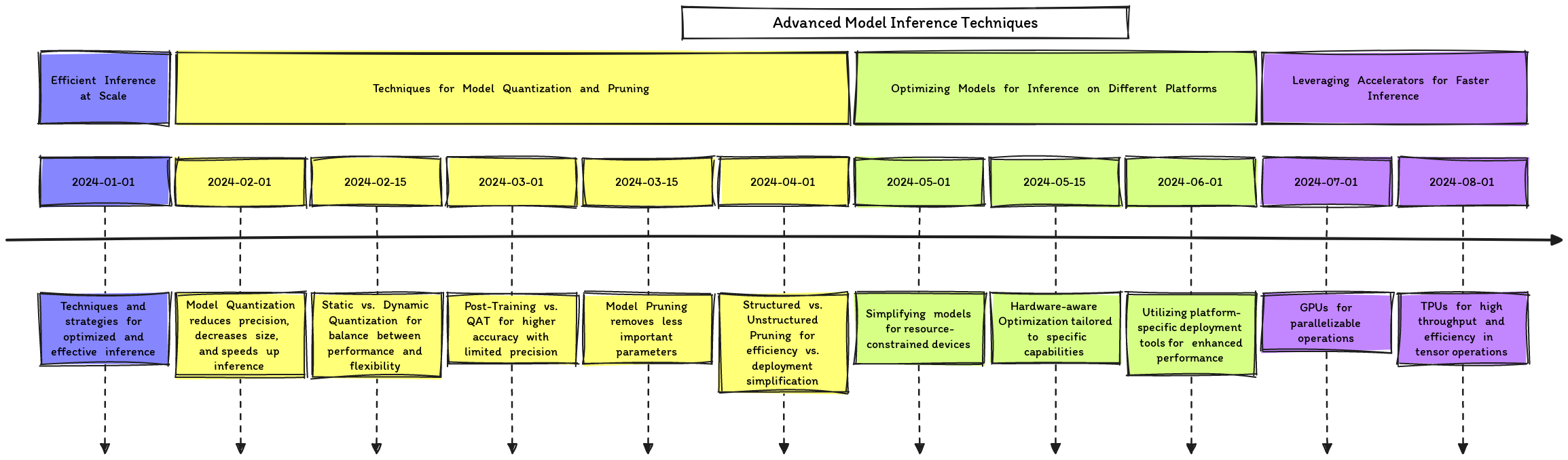
life cycle of optimizing for inference (From Sina Torfi — Open Source)
Let’s take a look at an example of LLM Inference optimization example:
<span id="025a" data-selectable-paragraph=""><span>import</span> torch<br><span>from</span> transformers <span>import</span> AutoModelForCausalLM, AutoTokenizer, BitsAndBytesConfig<br><span>import</span> time<br><br><span>def</span> <span>setup_model</span>(<span>optimized=<span>True</span></span>):<br> <br> tokenizer = AutoTokenizer.from_pretrained(<span>"facebook/opt-350m"</span>)<br><br> <span>if</span> optimized:<br> <br> quantization_config = BitsAndBytesConfig(<br> load_in_4bit=<span>True</span>,<br> bnb_4bit_compute_dtype=torch.float16<br> )<br> <br> model = AutoModelForCausalLM.from_pretrained(<br> <span>"facebook/opt-350m"</span>,<br> quantization_config=quantization_config<br> )<br> <br> model = model.to_bettertransformer()<br> <span>else</span>:<br> <br> model = AutoModelForCausalLM.from_pretrained(<span>"facebook/opt-350m"</span>)<br><br> <br> <span>return</span> tokenizer, model.to(<span>"cuda"</span>)<br><br><span>def</span> <span>generate_text</span>(<span>model, tokenizer, input_text, use_flash_attention=<span>False</span></span>):<br> <br> inputs = tokenizer(input_text, return_tensors=<span>"pt"</span>).to(<span>"cuda"</span>)<br><br> <span>if</span> use_flash_attention:<br> <br> <span>with</span> torch.backends.cuda.sdp_kernel(enable_flash=<span>True</span>, enable_math=<span>False</span>, enable_mem_efficient=<span>False</span>):<br> outputs = model.generate(**inputs)<br> <span>else</span>:<br> <br> outputs = model.generate(**inputs)<br><br> <br> <span>return</span> tokenizer.decode(outputs[<span>0</span>], skip_special_tokens=<span>True</span>)<br><br><span>def</span> <span>measure_performance</span>(<span>input_text, optimized=<span>True</span>, use_flash_attention=<span>False</span></span>):<br> <br> tokenizer, model = setup_model(optimized)<br><br> <br> start_time = time.time()<br><br> <br> result_text = generate_text(model, tokenizer, input_text, use_flash_attention)<br><br> <br> end_time = time.time()<br><br> <span>print</span>(<span>f"Generated Text: <span>{result_text}</span>"</span>)<br> <span>print</span>(<span>f"Time Taken: <span>{end_time - start_time:<span>.2</span>f}</span> seconds"</span>)<br><br><br>input_text = <span>"Hello my dog is cute and"</span><br><br><br><span>print</span>(<span>"Running optimized version:"</span>)<br>measure_performance(input_text, optimized=<span>True</span>, use_flash_attention=<span>True</span>)<br><br><br><span>print</span>(<span>"\nRunning unoptimized version:"</span>)<br>measure_performance(input_text, optimized=<span>False</span>, use_flash_attention=<span>False</span>)</span>
When your model is trained and ready, the next big step is making sure it works well in the real world.
Managing Latency and Throughput for Real-Time Applications
That means it should handle lots of requests, respond quickly, and stay reliable no matter what. Let’s look at how to efficiently scale your model inference in production.
In production, requests can come flying in fast. You want to spread these requests evenly across your servers so none of them get overloaded. This is what load balancing does it keeps everything running smoothly. But if it’s not done right, your system can still struggle.
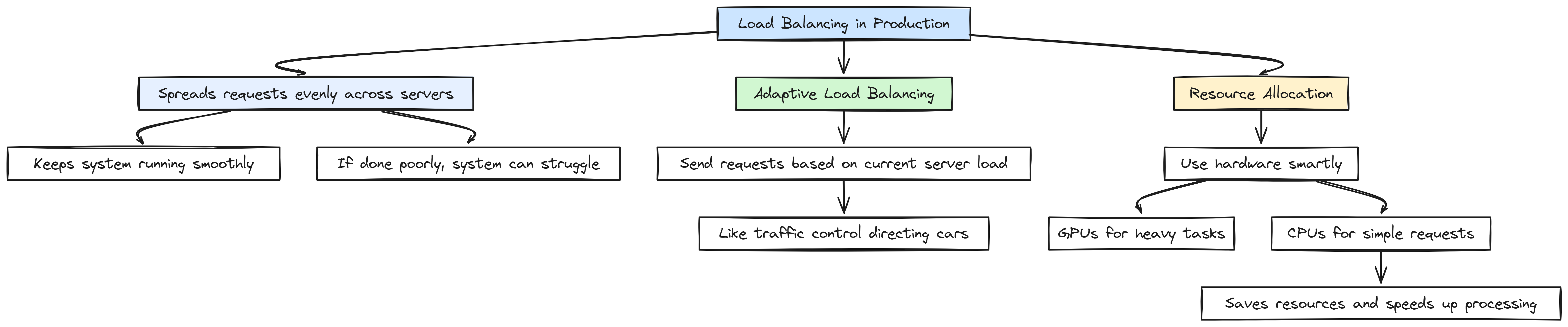
Load Balancing (Created by )
- Adaptive Load Balancing: This means sending requests to servers based on how busy they are at that moment like a traffic controller directing cars down the least crowded road.
- Resource Allocation: Using your hardware smartly matters a lot. GPUs are powerful for heavy tasks but can be overkill for simple requests. Assigning work to either GPU or CPU based on how demanding the request is helps save resources and speed things up.
<span id="8406" data-selectable-paragraph=""><span>import</span> torch<br><br><span>def</span> <span>allocate_inference</span>(<span>request</span>):<br> <span>"""Simple function to allocate inference to GPU or CPU based on request complexity."""</span><br> <br> <span>if</span> request.complexity > <span>5</span>:<br> device = torch.device(<span>"cuda:0"</span>) <br> <span>else</span>:<br> device = torch.device(<span>"cpu"</span>) <br> <br> <br> model = your_model.to(device)<br> <br> <br> <span>return</span> model</span>
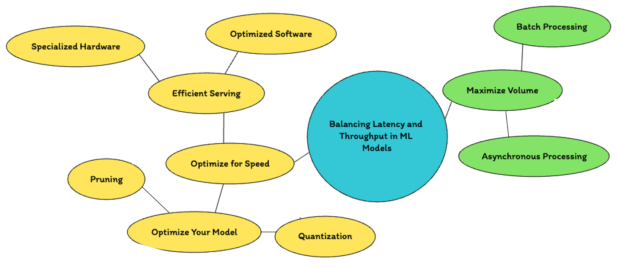
When your machine learning model goes live, especially in real-time apps, you’re juggling two big things: latency and throughput.
- Latency is how fast you get an answer back.
- Throughput is how many answers you can handle in a given time.
Zoom image will be displayed
Latency and Throughput (From Sina Torfi — Open Source)
Both matter a lot, but sometimes making one better can slow down the other. Let’s break down how to manage both without all the technical mumbo jumbo.
In real-time apps, users or systems don’t want to wait long. You want your model to give answers fast.
- Trim your model: Use techniques like quantization and pruning (covered earlier) to shrink your model and make it faster without losing accuracy.
- Serve smarter: The way you serve your model matters! Using GPUs when you need extra power or tools like TorchServe to efficiently manage requests can make a huge difference.
Throughput is about how many requests your model can handle at once, which matters a lot during traffic spikes.
- Batch Processing: Combine multiple incoming requests and process them together, like taking a bus full of passengers instead of a separate car for each person. It’s faster overall, but batches take a little time to fill up before they move.
- Asynchronous Processing: Let your system handle new requests while still working on previous ones like taking new orders while you’re still cooking. This keeps everything flowing smoothly.
Balancing latency and throughput means sometimes you need to change how many requests you process at once your batch size depending on what’s happening in real time.
Here is a simple way to do that with PyTorch:
<span id="e624" data-selectable-paragraph=""><span>import</span> torch<br><span>from</span> queue <span>import</span> Queue<br><span>from</span> threading <span>import</span> Thread<br><br><br>model = torch.nn.Linear(<span>10</span>, <span>2</span>)<br>model.<span>eval</span>() <br><br><span>def</span> <span>inference_worker</span>(<span>input_queue</span>):<br> <span>while</span> <span>True</span>:<br> <br> batch = input_queue.get()<br> <span>if</span> batch <span>is</span> <span>None</span>: <br> <span>break</span><br> <span>with</span> torch.no_grad(): <br> output = model(batch) <br> <br> input_queue.task_done() <br><br><br>input_queue = Queue(maxsize=<span>10</span>)<br><br><br>worker = Thread(target=inference_worker, args=(input_queue,))<br>worker.start()<br><br><br><span>for</span> _ <span>in</span> <span>range</span>(<span>100</span>):<br> input_batch = torch.randn(<span>5</span>, <span>10</span>) <br> input_queue.put(input_batch) <br><br>input_queue.put(<span>None</span>) <br>worker.join() </span>
So, far what we have learn so far …
It’s not just about speed or capacity it’s about balancing quick responses with smooth handling of heavy loads to keep users happy
Edge AI and Mobile Deployment
Deploying AI models on edge devices like smartphones and IoT gadgets means running AI right where the data is created.
This setup cuts down delays, saves network bandwidth, and keeps your data more private since it doesn’t have to leave the device.
To make AI work well on these limited devices, you need to focus on a couple of smart strategies:
- Model Optimization: Use techniques like quantization, pruning, and knowledge distillation to shrink your models. Smaller models run faster and fit better on less powerful hardware.
- Edge-Friendly Frameworks: Tools like TensorFlow Lite and PyTorch Mobile are built just for this. They help convert and optimize your models to run efficiently on edge devices.
<span id="981a" data-selectable-paragraph=""><span>import</span> tensorflow <span>as</span> tf<br><br><br>converter = tf.lite.TFLiteConverter.from_keras_model(model)<br>tflite_model = converter.convert()<br><br><span>with</span> <span>open</span>(<span>'model.tflite'</span>, <span>'wb'</span>) <span>as</span> f:<br> f.write(tflite_model)</span>
Edge devices often have tight limits on processing power, memory, and battery life. So your AI models need to be lean and efficient:
- Model Compression: Shrink your models using pruning or quantization to save space and speed up inference.
- Energy-Efficient Algorithms: Pick or design algorithms that don’t drain the battery or overload the processor.
- Edge-Optimized Architectures: Use networks like MobileNet or EfficientNet, built specifically to be fast and light while still accurate.
Phase IV: Performance Analysis and Optimization
When optimizing AI systems, it’s key to spot where things slow down the bottlenecks so you can fix them and boost performance.
Diagnosing System Bottlenecks
Two main tools to help here are profiling and benchmarking.
Profiling is about digging deep to see how your system uses resources like CPU, GPU, and memory, and how long different parts of your code take to run. It’s like having a performance map that highlights the slow or heavy spots you want to improve.
- Python’s cProfile: A handy built-in tool to measure where your Python code spends most of its time.
- NVIDIA Nsight Systems: If you use NVIDIA GPUs, this tool tracks GPU performance and helps find bottlenecks in CUDA code.
Benchmarking looks at the bigger picture: how fast and efficient your whole system is compared to standards or past versions. It sets a baseline, so you know where you started and can measure how much your changes help.
- Establish Baselines: Benchmark your current system before changing anything.
- Compare: Check how your system stacks up against others or industry benchmarks.
- Measure Impact: After optimizations, benchmark again to see if your improvements really made a difference.
Bottlenecks come in different forms like compute, memory, or network and each needs different fixes.
Compute Bottlenecks happen when your processor (CPU/GPU) can’t keep up with the work.
Fixes:
- Use parallel computing: Spread work across multiple cores or GPUs to speed things up.
- Optimize algorithms: Simplify calculations or switch to more efficient methods to lighten the load.
Memory Bottlenecks happen when your system can’t move data fast enough or runs out of memory.
Fixes:
- Cache frequently used data to avoid slow memory reads.
- Reduce your memory footprint using pruning, quantization, or lighter data structures.
- Example: If your model’s too big for GPU memory, you might need these tricks since you can’t just add more RAM.
Network Bottlenecks Show up in distributed systems where data needs to travel between machines.
Fixes:
- Use better data serialization to shrink the size of data being sent.
- Switch to more efficient communication protocols that lower latency and speed up data transfer.
Operationalizing AI Model
Keeping an eye on both your system’s health and your AI model’s performance is critical for smooth, reliable operations. Good monitoring helps catch problems early before they turn into bigger issues. Here’s a straightforward approach to setting up an effective monitoring strategy:
Tools you can use:
Zoom image will be displayed

- Prometheus: An open-source tool that collects and stores metrics like CPU usage, memory consumption, disk I/O, and network traffic. It’s great for tracking the overall health of your AI infrastructure.
- Grafana: A powerful visualization tool that works well with Prometheus to create intuitive dashboards. It helps spot anomalies and trends in your system data easily.
Model Performance Monitoring Popular options include:
- TensorBoard: Built for TensorFlow and PyTorch, TensorBoard lets you visualize training and evaluation metrics like loss, accuracy, weight distributions, and even your model’s architecture. Regularly checking these helps you understand how your model is learning and performing.
- Custom Logging: Sometimes you’ll need to track metrics or events specific to your application that TensorBoard doesn’t cover. Implementing your own logging system lets you capture predictions, errors, or any custom KPIs for deeper analysis.
So, some of the best monitoring techniques are:
Zoom image will be displayed
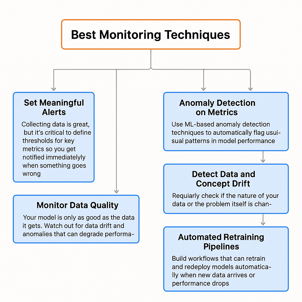
Best Monitoring Techniques (Created by )
- Set Meaningful Alerts: Collecting data is great, but it’s critical to define thresholds for key metrics so you get notified immediately when something goes wrong. Alerts help you act fast before issues impact users.
- Monitor Data Quality: Your model is only as good as the data it gets. Watch out for data drift (changes in input data over time) and anomalies that can degrade performance. For example, logging sample images or data batches can help you detect shifts early.
- Continuous Evaluation: Keep evaluating your model with fresh data regularly to spot performance drops. Automate alerts or retraining triggers when accuracy or other metrics fall below set thresholds, ensuring your model stays effective.
- Anomaly Detection on Metrics: Use ML-based anomaly detection techniques to automatically flag unusual patterns in model performance, so you’re always on top of potential issues without manual inspection.
- Detect Data and Concept Drift: Regularly check if the nature of your data or the problem itself is changing. Dedicated drift detection tools can alert you to these shifts, prompting model updates or retraining.
- Automated Retraining Pipelines: Build workflows that can retrain and redeploy models automatically when new data arrives or performance drops. But be smart set strict criteria to avoid wasting resources on tiny improvements that don’t matter much in practice.
Debugging AI Systems: Tools and Methodologies
Debugging AI is tricky due to complex data flows and models. Use these tools and approaches:
Zoom image will be displayed

- PyTorch Autograd Profiler: Checks time and memory usage in PyTorch models.
- TensorFlow Debugger (tfdbg): Inspects tensor values to spot errors like NaNs or wrong shapes.
- Interactive Debugging: Use Jupyter notebooks for real-time data and model checks.
- Advanced Profiling: Tools like NVIDIA Nsight and PyTorch Profiler analyze GPU use and hardware bottlenecks to optimize performance.
CI/CD Pipelines for Machine Learning
Fast, reliable model updates are key in AI projects. CI/CD automates testing, integration, and deployment to keep models working smoothly with minimal manual effort.
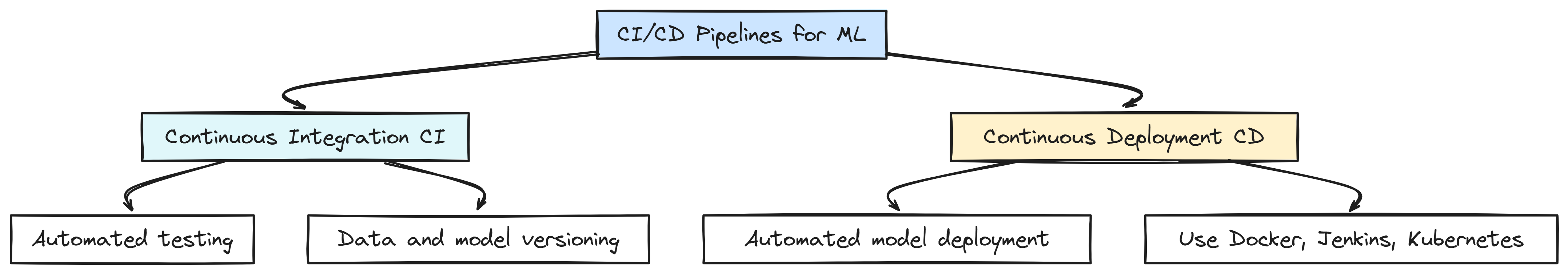
CI/CD Pipeline (Created by )
Being able to quickly test and improve ML models is key to building successful AI systems. By using CI/CD (Continuous Integration and Continuous Deployment), we can automate testing, model updates, and deployment with minimal manual effort. This keeps everything running smoothly and reliably.
Continuous Integration (CI) in ML
CI means automatically checking code changes to catch issues early. In ML, it also includes checking data, training scripts, and the models themselves.
- Automated Testing: Set up tests to check data quality, model training, and predictions. Use unit tests for small parts and integration tests for full pipelines.
- Version Control: Use tools like DVC to track changes in data and models, just like with code. This helps keep everything consistent and easy to roll back if needed.
Continuous Deployment (CD) in ML
CD means automatically putting new models into production so users get the latest improvements quickly.
- Model Serving: Tools like TensorFlow Serving or TorchServe help serve models efficiently and manage versions.
- Docker: Use Docker to bundle your model with all its dependencies. This makes it easy to run the model anywhere.
- Jenkins + Kubernetes: Use Jenkins to automate tasks like testing and deploying models. Combine with Kubernetes to scale and manage models in production.
Extra Tools to Make It Work Better
- Experiment Tracking: Tools like MLflow or Weights & Biases help track experiments, model metrics, and results.
- Environment Management: Use tools like Conda or Pipenv to manage Python packages, and pair with Docker for consistency across development and production.
- Model Validation: Set up automated checks to make sure each model meets performance standards (e.g., accuracy or precision) before deploying.
Conclusion
Thanks for reading! I hope this guide helps you with your AI work, whether you’re starting something new or improving what you already have. AI works best when people share and learn together.
If you have ideas or projects, feel free to share them!